Lab Review
Lab 1:
To begin our 479 Labs, we started by investigating the prevalence of Heart Diseases in the Southern US. Using CDC Wonder Data and ArcMap’s model builder we highlighted the heart disease hot spots between 1999 and 2016. In many ways, to me this lab acted like a refresher course on the basics of Spatial Analysis and how to use ArcMap. We concluded that counties that were considered to have a high rate of heart diseases were also found to be spatially correlated with one another. It has admittedly been some time since I have last created maps on ArcMap so I was a little rusty with all of the tools. This reflected in my work as you can see that my first map created for this course was evidently lacking. Regardless this lab was an excellent first step into getting back into the groove of using GIS software.
Map 1: Map of the 2010 Heart Disease Hot Spots located in the Southern US. (This map did not properly show the hot spots and was evident that my work needed to be improved upon.)
Lab 2:
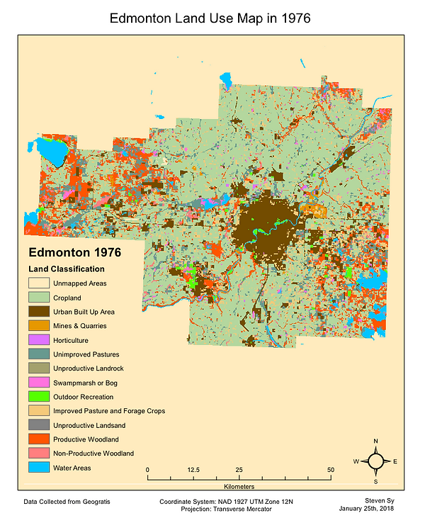
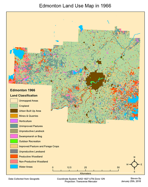
Our second lab was focused on exploring the statistical analysis program, FragStats, by analyzing the land use around Edmonton, Alberta. We were placed in a position of a consultant tasked with writing a report on the state of the local landscape based on the changes between 1966 and 1976. We collected data from Geogratis, ran the metrics through FragStats and created a Transition Matrix to aid in our understanding of how the land was being used. In our analysis, we concluded that much of the area had been converted from croplands into urbanized developments. While the downtown Edmonton core saw a large expansion, there were also positive signs that environmental conservation strategies were proving effective as productive woodlands increased by about 12,000 hectares.
Map 1: Map showing the Land Use of the Edmonton, Alberta Region in 1966.
Map 2: Map showing the Land Use of the Edmonton, Alberta Region in 1976.
Lab 3:
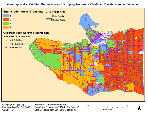
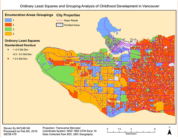
For the third lab of this course we looked at how a Geographically Weighted Regression (GWR) analysis can be applied to investigate the effects of local relations between childhood development variables in Vancouver. We assessed how different factors like income, households of single parents and dependence on childcare would affect a child’s social skills, language abilities and physical strengths. We arranged the enumeration areas into groups of similar characteristic neighborhoods then performed an Ordinary Least Squares analysis on the development variables. The Vancouver East Side was largely dominated by low income, single parent families while the Downtown core and Western Region of Vancouver were largely occupied by fairly wealthy, small families that do not depend on childcare. Through our GRW analysis, we found that language proficiency and gender had a strong correlation to accurate analyses of Early Childhood Development while income levels showed very little relationship to Childhood social skills.
Map 1: Ordinary Least Squares compared to Grouping Analysis results.
Map 2: Geographically weighted Regression compared to Grouping Analysis results.
Lab 4:
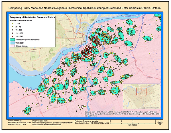
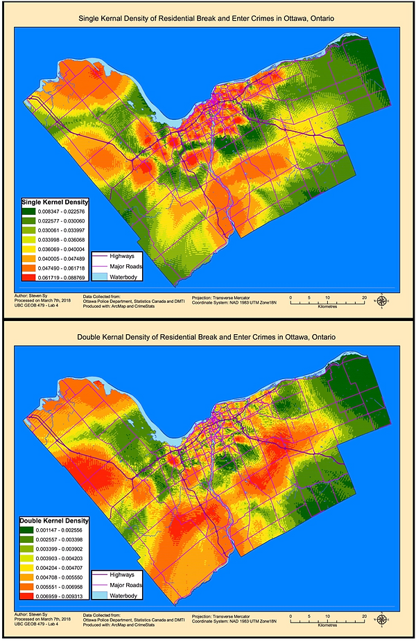
In our fourth and final lab for GEOB 479, we investigated the spatial and temporal relationships between crime events in the Nepean, Ottawa region between Jan 2005 and March 2006. By using a program called Crime Stats we analyzed how car thefts, residential and commercial breaking and entering crimes were clustered throughout the region. In our analysis, we identified crime hot spots and created kernel density maps to show areas with the highest risk of a crime occurring. We learned that zoning laws can greatly influence how certain environments are susceptible to behavioral patterns. Commercial and residential areas demonstrate a strong clustering of crime events. This lab identified the dangers of simply looking at the raw numbers of crimes to identify areas of concern for police officers. We need to use relative stats like density of crimes to get a better sense of the context that these crimes are occurring in. We could discern that Downtown Ottawa might have a higher number of crime events because there simply more people that visit the area and that it may not be accurate for police for officers to deem the area as risky. This lab showed that there a number of ways to look at an existing problem and each method of analysis reveals an important information. As GIS analysists, it is important to consider this as we take on our own research projects.
Map 1: Map comparing the nearest neighbour hierarchical spatial clusters of residential break and enter crimes to the distribution of residential break and enter crime hot spots in central Nepean, Ottawa between Jan 2005 and March 2006.
Map 3 and 4: Comparison maps of the singel (top) and double (bottom) kernel density of residential break and enter crimes in Nepean, Ottawa between Jan 2005 & March 2006.